Diagnostic Modeling
For Educational and Psychological Assessment
W. Jake Thompson, Ph.D.
Who am I?
W. Jake Thompson, Ph.D.
- Assistant Director of Psychometrics
- ATLAS | University of Kansas
- Research: Applications of diagnostic psychometric models
- Lead psychometrician and Co-PI for the Dynamic Learnings Maps assessments
- PI for an IES-funded project to develop software for diagnostic models
Acknowledgements
The research reported here was supported by the Institute of Education Sciences, U.S. Department of Education, through Grant R305D210045 to the University of Kansas. The opinions expressed are those of the authors and do not represent the views of the the Institute or the U.S. Department of Education.

Diagnostic assessments
What is an assessment?
- Social sciences are often interested in latent variables
- Math knowledge
- Psychopathology
- Personality traits
- Assessments are designed to measure the unmeasurable
- Educational assessment
- Psychological screening tools
- Personality questionnaires
- Today’s example: A test on musical knowledge
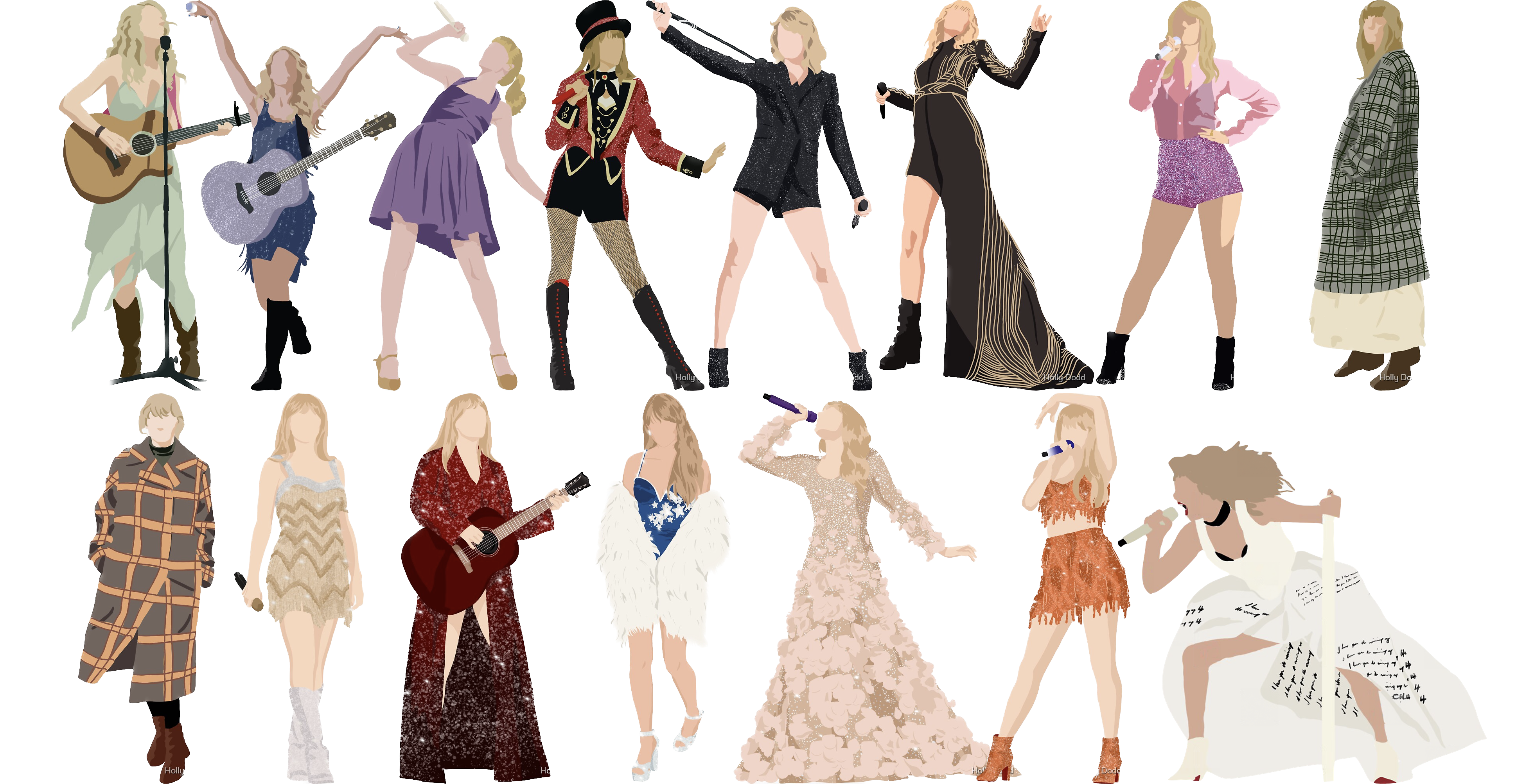
- Traditional assessments and psychometric models measure an overall skill or ability
- Assume a continuous latent trait
Traditional measurement
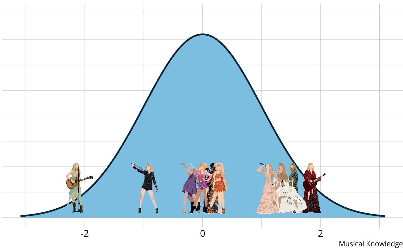
- The output is a weak ordering of eras due to error in estimates
- Confident Taylor Swift (debut) is the worst
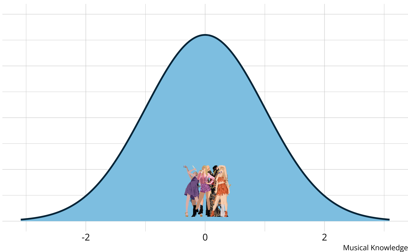
- Not confident on ordering toward the middle of the distribution
- Limited in the types of questions that can be answered.
- Why is Taylor Swift (debut) so low?
- What aspects do each era demonstrate proficiency or competency of?
- How much skill is “enough” to be competent?
Diagnostic measurement
- Designed to be multidimensional
- No continuum of student achievement
- Categorical constructs
- Usually binary (e.g., master/nonmaster, proficient/not proficient)
- Several different names in the literature
- Diagnostic classification models (DCMs)
- Cognitive diagnostic models (CDMs)
- Skills assessment models
- Latent response models
- Restricted latent class models
Diagnostic music assessment
- Rather than measuring overall musical knowledge, we can break music down into set of skills or attributes
- Songwriting
- Production
- Vocals

- Attributes are categorical, often dichotomous (e.g., proficient vs. non-proficient)
DCMs in practice
Benefits
- Fine-grained, multidimensional results allow us to answer more questions
- Why is Taylor Swift (debut) so low?
- What aspects of musical knowledge had demonstrated proficiency in each era?
- Incorporates complex item structures
- High reliability with fewer items
Applications
- Not often used for practical applications
- Software constraints
- Only estimate restrictive DCMs
- Limited functionality for model evaluation

Data requirements
#> # A tibble: 502 × 22
#> album `1` `2` `3` `4` `5` `6` `7` `8`
#> <chr> <int> <int> <int> <int> <int> <int> <int> <int>
#> 1 Taylor Swift 0 0 0 0 0 0 0 0
#> 2 Fearless 1 0 1 0 0 0 0 0
#> 3 Fearless (Taylor's Version) 1 1 0 1 0 0 0 1
#> 4 Speak Now 1 0 1 0 0 0 0 0
#> 5 Speak Now (Taylor's Version) 1 0 0 1 1 0 0 0
#> 6 Red 1 1 0 0 1 1 1 0
#> 7 Red (Taylor's Version) 1 1 0 1 1 1 1 1
#> 8 1989 0 1 0 0 0 1 1 0
#> 9 1989 (Taylor's Version) 1 1 0 1 1 1 1 0
#> 10 reputation 0 1 1 0 1 0 0 1
#> # ℹ 492 more rows
#> # ℹ 13 more variables: `9` <int>, `10` <int>, `11` <int>, `12` <int>,
#> # `13` <int>, `14` <int>, `15` <int>, `16` <int>, `17` <int>, `18` <int>,
#> # `19` <int>, `20` <int>, `21` <int>Model estimation
taylor_lcdm <- measr_dcm(
data = taylor_data, qmatrix = taylor_qmatrix,
resp_id = "album",
type = "lcdm",
method = "mcmc", backend = "rstan",
warmup = 1000, iter = 1500,
chains = 2, cores = 2,
file = here("fits", "taylor-lcdm")
)- 1
- Specify your data, Q-matrix, and ID columns
- 2
- Choose the DCM to estimate (e.g., LCDM, DINA, etc.)
- 3
- Choose the estimation engine
- 4
- Pass additional arguments to rstan or cmdstanr
- 5
- Save the model to save time in the future
Respondent probabilities
#> $class_probabilities
#> # A tibble: 4,016 × 5
#> album class probability `5.5%` `94.5%`
#> <fct> <chr> <dbl> <dbl> <dbl>
#> 1 Taylor Swift [0,0,0] 9.97e- 1 9.95e- 1 9.99e- 1
#> 2 Taylor Swift [1,0,0] 4.28e- 5 1.52e- 5 9.03e- 5
#> 3 Taylor Swift [0,1,0] 1.44e- 3 4.61e- 4 3.04e- 3
#> 4 Taylor Swift [0,0,1] 1.44e- 3 4.92e- 4 2.89e- 3
#> 5 Taylor Swift [1,1,0] 4.84e- 9 5.79e-10 1.47e- 8
#> 6 Taylor Swift [1,0,1] 8.40e- 9 1.45e- 9 2.11e- 8
#> 7 Taylor Swift [0,1,1] 3.80e- 6 7.81e- 7 9.54e- 6
#> 8 Taylor Swift [1,1,1] 7.93e-13 5.16e-14 2.54e-12
#> 9 Fearless [0,0,0] 3.82e- 1 1.84e- 1 6.16e- 1
#> 10 Fearless [1,0,0] 6.01e- 1 3.58e- 1 8.06e- 1
#> # ℹ 4,006 more rows
#>
#> $attribute_probabilities
#> # A tibble: 1,506 × 5
#> album attribute probability `5.5%` `94.5%`
#> <fct> <chr> <dbl> <dbl> <dbl>
#> 1 Taylor Swift songwriting 0.0000428 0.0000152 0.0000903
#> 2 Taylor Swift production 0.00144 0.000462 0.00305
#> 3 Taylor Swift vocals 0.00144 0.000493 0.00290
#> 4 Fearless songwriting 0.603 0.365 0.810
#> 5 Fearless production 0.0111 0.00316 0.0250
#> 6 Fearless vocals 0.00631 0.00210 0.0132
#> 7 Fearless (Taylor's Version) songwriting 0.992 0.983 0.998
#> 8 Fearless (Taylor's Version) production 0.00106 0.000220 0.00271
#> 9 Fearless (Taylor's Version) vocals 0.152 0.0385 0.337
#> 10 Speak Now songwriting 0.603 0.365 0.810
#> # ℹ 1,496 more rowsProbabilities to profiles
| album | songwriting | production | vocals | |
|---|---|---|---|---|
Taylor Swift |
||||
Fearless |
||||
Speak Now |
||||
Red |
||||
1989 |
||||
reputation |
||||
Lover |
||||
folklore |
||||
evermore |
||||
Fearless
Taylor's Version
|
||||
Red
Taylor's Version
|
||||
Midnights |
||||
Speak Now
Taylor's Version
|
||||
1989
Taylor's Version
|
||||
THE TORTURED POETS |
- No scale, no overall “ability”
- Feedback on specific skills as defined by the cognitive theory and test design
Fine-grained feedback
- Distinguish between respondents who may have similar scale scores
| album | songwriting | production | vocals | |
|---|---|---|---|---|
Fearless |
||||
Speak Now |
||||
Red |
||||
reputation |
||||
Lover |
||||
evermore |
||||
Fearless
Taylor's Version
|
||||
1989
Taylor's Version
|
Model evaluation
#> # A tibble: 1 × 3
#> m2 df pval
#> <dbl> <int> <dbl>
#> 1 183. 162 0.121When are DCMs appropriate?
Success depends on:
- Domain definitions
- What are the attributes we’re trying to measure?
- Are the attributes measurable (e.g., with assessment items)?
- Alignment of purpose between assessment and model
- Is classification the purpose?
When are DCMs not appropriate?
When the goal is the ordering of individuals on a scale
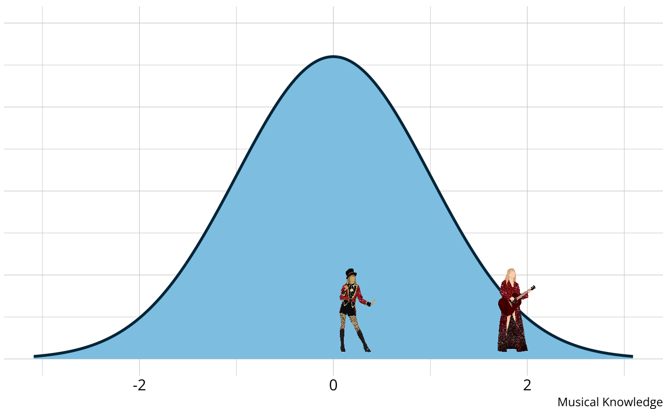
DCMs do not distinguish within classes
| album | songwriting | production | vocals | |
|---|---|---|---|---|
Red |
||||
Red
Taylor's Version
|
Learn more about DCMs
Learn more about measr
Thank you!
Slides
